This chapter discusses MW Profiler-the application you use to view the data created by the CodeWarrior profiler.
In this chapter you will look at:
The MW Profiler viewer application displays profiler output for you to analyze the results of your program's execution. MW Profiler reads the profiler dump files created by the calls in your code and displays the data in a form that you can use. Using the data display you can:
The MW Profiler application is very easy to use.
You open profile data files exactly as you open files in any application. You can use the Open... command from the MW Profiler File menu or drop the data file's icon on the MW Profiler icon. Whatever approach you take, when you open a file a window appears.
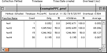
MW Profiler allows you to view several elements of the profile data simultaneously, as shown in Figure 4.1.
MW Profiler allows you to view summary data, detailed data, or object-based data. All three ways of viewing data use the same window shown in Figure 4.1. The display of the contents changes slightly for the different views.
See also "Window Views."
At the top of the window is a line with information about the data on display. The figure shows four items, but six are possible. What they are and what they represent is listed in Table 4.1.
| Item |
Contents |
|---|---|
The last two items-OverflowStack and OverflowFunctions-only appear
if the parameters you passed to ProfilerInit() did not create a buffer large enough to hold all the collected
data.
The OverflowStack number includes duplicate routine calls. If
it is small, it is the amount by which you should increase the
stackDepth parameter in the call to ProfilerInit(). If it is large, increase the value of the stackDepth parameter by some increment and try again.
The OverflowFunctions number also includes duplicate routine calls.
It is likely to be much larger than the size by which you need
to increase the numFunctions parameter in the call to Profiler-Init(). It might even be in the thousands.
If either overflow occurs, just increase the value of the respective
parameter in the ProfilerInit() call so the profiler allocates a larger data buffer.
Below the header information is a series of columns containing data from the profile. All times are displayed according to the resolution of the timer that you use to profile data. The results in the window are only as precise as the timer used.
The times shown in the data columns are displayed in milliseconds.
A millisecond (ms) is one thousandth of a second. Each time datum
is reported to three decimal places. This gives you microsecond
results. A microsecond (µs) is one thousandth of a millisecond,
or one millionth of a second. However, some time bases (most notably
ticksTimeBase) are less precise. Ticks increment 60 times a second. See "Time and Timebases."
Figure 4.1 does not show all the data columns. You can scroll to see the columns beyond the right edge of the window. You can also resize the columns to get more information in the window.
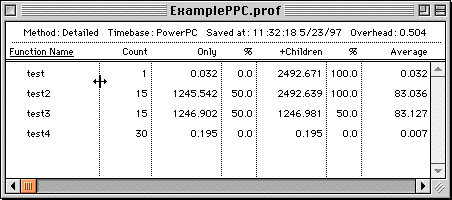
Move the cursor over one of the column lines. The cursor changes to a directional arrow, as shown in Figure 4.2. Click and drag the column line to where you want it.
Table 4.2 lists each of the columns in the profiler window (from left to right) and the information that column contains.
| Column |
Contents |
|---|---|
 NOTE
NOTE If you're profiling Mac OS code, you should know that there is a slight difference between the 68K and the PowerPC in the stack tracking code. On a 68K machine the profiler is called before a routine sets up its stack. Therefore, the stack values that a 68K profile reports do not include the called routine's stack. On a PowerPC, the profiler is called after a routine sets up its stack. Therefore, the stack values on a PowerPC profile do include the called routine's stack.
You can view the data sorted by the value in any column. Names are listed alphabetically from top to bottom, numbers are listed from greater to lesser.
To change the sort order, either click the column title, or choose a menu item from the View menu. The heading becomes underlined and data is sorted by the value in that column.
If you wish to export information from the results, use the Save As... command in the File menu. This saves all the data in a tab-delimited text file. The text file is organized the same way that the window is organized.
You can open any number of different profile windows simultaneously, limited only by the MW Profiler's memory allotment. This allows you to compare the results of different runs easily.
In the MW Profiler View menu you may choose to view the data in one of three ways: summary, detailed, or object. Not all possibilities are available for all profiles.
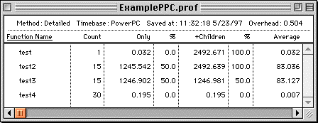
The summary view displays a complete, non-hierarchical, flat list of each routine profiled. No matter what calling path was used to reach a routine, the profiler combines all the data for the same routine and displays it on a single line. Figure 4.3 shows a summary view.
The summary view is particularly useful for comparing routines to see which take the longest time to execute. The summary view is also useful for finding a performance problem with a small routine that is called from many different places in the program. This view helps you look for the routines that make heavy demands in time or raw number of calls.
A summary view window can be displayed for any profile.
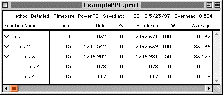
The detailed view displays routines according to the dynamic call tree as shown in Figure 4.4.
Routines that are called by a given routine are shown indented under that routine. This means that a routine may appear more than once in the profile if it called from different routines. This makes it difficult to tell how much total time was spent in a routine. However, you can use the summary view for that purpose.
The detailed view is useful for detecting design problems in code. MW Profiler in detailed view lets you see what routines are called how often from what other routines. Armed with knowledge of your code's underlying design, you may discover flow-control problems.
For example, you can use detailed view to discover routines that are called from only one place in your code. You might decide to fold that routine's code into the caller, thereby eliminating the routine call overhead entirely. If it turns out that the little routine is called thousands of times, you can gain a significant performance boost.
You can use the Expand All or Collapse All commands in the View menu to open or close the entire hierarchy at once.
In detailed view, sorting is limited to routines at the same level in the hierarchy. For example, if you sort by routine name, the routines at the top of the hierarchy will be sorted alphabetically. For each of those first-level routines, its second-level routines will be sorted alphabetically underneath it, and so on.
The detailed view requires that collectDetailed be passed to ProfilerInit() when collecting the profile. If collectSummary is used, you cannot display the data in detailed view.
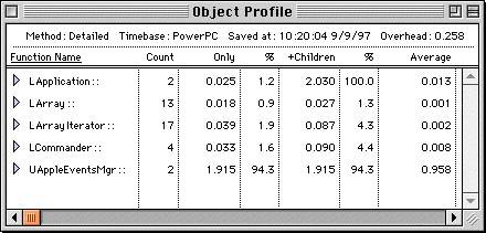
The object view displays summary information sorted by class. Beneath each class the methods are listed. This is a two-level hierarchy. You can open and close a class to show or hide its methods, just like you can in the detailed view.
When sorting in object view, functions stay with their class, just like subsidiary functions in detailed view stay in their hierarchical position. Figure 4.5 shows the methods sorted by count.
Object view allows you to study the performance impact of substituting one implementation of a class for another. You can run profiles on the two implementations, and view the behavior of the different objects side by side. You can do the same with the summary view on a routine-by-routine basis, but the object view gives you a more natural way of accessing object-based data. It also allows you to gather all the object methods together and view them simultaneously, revealing the effect of interactions between the object's methods.
Object view will display "N/A" (Not Available) in the +Children
column for classes in a collectSummary profile. This is because the detail information is missing from
the file.
The object view requires that the profile contain at least one mangled C++ name. If there is none, you cannot use object view.
As you work with MW Profiler, you will see that the information provided quickly guides you to problem areas.
To look for time hogs, sort the view by either the Only column or the +Children column. Then examine routines that appear near the top of the list. These are the routines that swallow the greatest percentage of your code's time. Any improvement in these routines will be greatly magnified in your code's final performance.
You may also want to sort based on the number of times a routine is called. The time you save in a heavily-used routine is saved each time it is called.
If stack size is a concern in your code, you can sort based on the Stack Space column. This lets you see the largest size the stack reached during the profile. Remember that in Mac OS 68K code the stack for the called routine is not included in the Stack Space data.